Animations: not so difficult after all

Creating simple animations is not as difficult as you may think. Graphic designer, scientist, and science communicator Szymon Drobniak shares a range of tools and approaches – from graphic software to R – along with tutorials and inspirations to get you started with creating moving images and graphs.
Many scientists consider making their own illustrations for slides and posters an impossible task. The usual perception is that you need lots of talent, knowledge of some super difficult graphical software – and time. The truth is, that actually only this last thing may be a decisive factor – it turns out that producing simple and captivating illustrations is not very difficult. Thanks to modern graphical software it does not require much of drawing skills. Of course, having your first moments with Adobe Photoshop or Illustrator may be intimidating – these programs are really accessible and easy to master, at least in the extent necessary to produce nice and esthetic visuals. What are the benefits? Most importantly: more control over the appearance of your illustrations and the way they are reproduced in your publications.
It’s not surprising that if illustration-making is not so popular – animating your visuals seems even more difficult. Making “moving images” seems a very advanced skill – but bear in mind that no one expects you to produce cartoons like those from the Pixar Studio. Animating simple biochemical processes or adding motion to simple shapes is an easy and powerful way of adding them this additional dimension.
The important question is – what software to use? The choice depends on the final product that you’d like to achieve. Here’s a couple of tools you might have a go at.

“Hand drawn” animations with VideoScribe
You might know “Minute Physics” – an excellent YouTube channel explaining some difficult concepts in modern physics with captivating “hand drawn” animations. The hardware behind creating these wonderful videos is old-school film making using a digital camera and a special mini studio. It turns out, you can easily achieve similar results using VideoScribe. It’s a tool that turns existing line drawings into animated hand drawing movies. You need existing images, or some visuals which you draw yourself, either digitally or on paper. Then you can get them moving with VideoScirbe. Studies show, that identical content presented as still images vs. animated drawings has a much bigger chances of being assimilated by the audience when presented as animated cartoons.

Pencil2D – open source animation software
Finding the right tool to create your first animation from scratch may be a difficult task – free alternatives are not very impressive, usually have pretty steep learning curves and require you to switch to a whole new way of working with images. One exception that deserves attention is Pencil – a very simple-looking, but very powerful tool for creating 2D animations. It has a very rich set of options, and an excellent community of supporters that share their experience with newbies.

Adobe Creative Cloud and (surprisingly) Photoshop
On an everyday basis I work with programs from the Adobe Creative Cloud. The principal tool for creating animated movies within this package is Adobe AfterEffects. Explaining the power of AfterEffects is beyond the scope of this short post. However, it turns out that even Adobe Photoshop – a photo-editing program designed for manipulating bitmap pictures – can be used to animate. The great thing about it is that the whole process is easy enough even for an inexperienced user. My adventure with Photoshop animation started after watching these animated infographics (follow links to see them):
An animated guide to breathing
The author of these animations, Eleanor Lutz, is a scientist and a graphic designer. As a designer she specializes in creating captivating animated information summaries. What is even more astonishing – she creates all of her animations in Adobe Photoshop – a software that was not designed to create such outputs. I could write a long tutorial myself here but let’s give space to Eleanor – on her website she posted a very good introduction to how to use Photoshop to animate shapes and colours (follow the link below).
Tutorial: “How to make an animated infographic” by Eleanor Lutz
The procedure is straightforward. Before starting, there are three things you have to familiarize yourself with:
- You have to understand layers, which are stacked portions of content, each covering what is beneath it. Eleanor uses layers to create separate frames of her animations.
- You should know how to draw and create colours in Photoshop. Basically there are two choices: either use the Brush tool (brush-looking icon on the right left-hand side of the window) or create simple geometrical shapes that you can then modify and distort (using the Shape tool (rectangle/ellipse icon) or the Pen tool (pen-shaped icon). Using either brush or shape-making tools you can easily control their colours through the colour palette visible as a coloured square below the column of icons on the left.
- Although Photoshop gives you hundreds of fancy special effects (found in the Filters menu) – don’t use them. If you’re starting with Photoshop – it’s best to keep things simple and use few colours, simple bold shapes and no distracting blurred gradients that would only obscure your first images.
Other than these three remarks – just follow Eleanor’s tutorial and I guarantee that you’ll be taken at once by the power of simple GIF animations.
An important question arises: where to get Photoshop? The sad truth is that this software is not free. Some Universities maintain an institutional licence for Adobe CC – you have to check it yourself to be sure. However, nowadays the academic license for Adobe CC (including Photoshop, Illustrator, AfterEffects and Acrobat Pro) costs only about 20 Euro per month (depending on your country). If you really think that science illustration is something you’d like to explore more – it’s not a very discouraging price tag…

Going wildeR – animation with R
Software used by graphic designers is not the only way of getting an animated output for your data. It turns out that even hard-core statistical computing programs can use the power of animation – the only question is how get it. My favourite candidate here is R – a free open-source computing environment, with tons of cool and useful packages that expand its functionality, created by the R community.
One of the packages is called “animation” and it enables the creation of animated figures straight from within R. The whole process is very simple and has only few difficulties. We will follow it trying to visualize two differing animation tasks.
First – install the package within R:
install.packages(“animation”)

library(“animation”)
In order for the package to work, you also have to install ImageMagic – a collection of libraries used by ‘animation’ to convert still images to GIFs. If you’d like to use movie clips (e.g. AVI) instead of GIFs – ‘animation’ lets you do this, but first you have make sure you have the latest ffmpeg library installed in your system. To download and install ImageMagic visit http://www.imagemagick.org.
For our first task we will animate a derivative of a function – in this tutorial this will be a quadratic function f(x) = 10x2+5x-6. Let’s define this equation first using R’s function definition syntax:
func <- function(x) {10*x^2+5*x-6}
In exactly the same way you can define any function of x, just place relevant operations within the curly brackets above. We can now plot our quadratic curve and add to it an arbitrary point at x = 4 (where in a moment we will calculate the function’s derivative).
curve(func, from=0, to=10, col=“blue”, lwd=3)

x0 <- 4
points(x0, func(x0), cex=2, col=“red”)
Now let’s plot a simple derivative of this function at a given poin x0. To do this we will need the ‘numDeriv’ package, if you don’t have it – you’ll have to install it. We first load the package:
library(numDeriv)
and calculate the slope of the derivative (or – in other words – the angle of the tangential line “touching” the plot at a given x0):
slope <- grad(func, x0)
The intercept of the tangential can be easily calculated knowing the x0, the slope and the value of our quadratic curve at x0:
intercept <- func(x0) - slope*x0
Finally let’s add the tangential line (which illustrates the derivative) to the plot:
abline(a=intercept, b=slope, col=“red”, lwd=2)
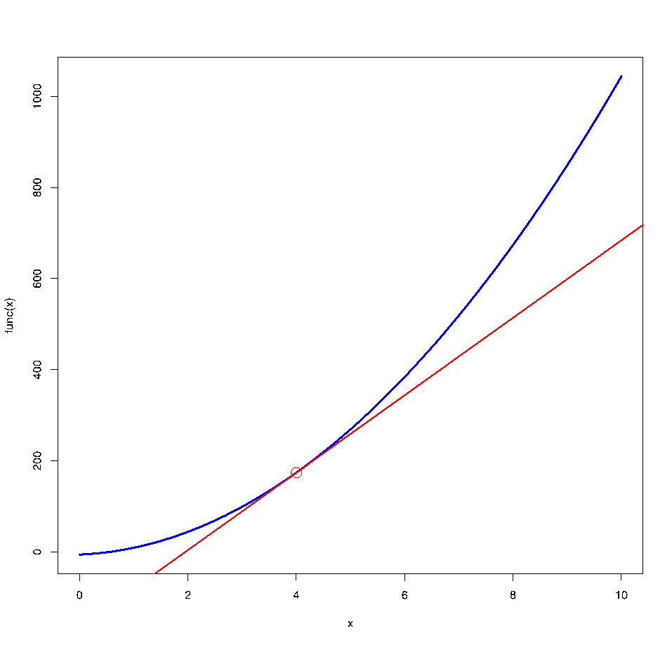
Now the trick is to make the red circle – and it’s associated tangential – moving along the blue quadratic curve. In order to achieve this we will use the saveGIF function from the ‘animate’ package. Inside of this function we will define a ‘for’ loop that will call values between 0.25 and 10 (in 0.25 increments). In each step of the loop the selected value will be used as a new x0 – which will basically “sweep” the tangential along the curve within the plotted range of 0 to 10.
x0 <- 0
saveGIF({
for(i in seq(0.25,10,0.25)){
## plot of a derivative
func <- function(x) {10*x^2+5*x-6}
curve(func, from=0, to=10, col=“blue”, lwd=3)
points(x0, func(x0), cex=2, col=“red”)
library(numDeriv)
grad(func, x0) -> slope
intercept <- func(x0) - slope*x0
abline(a=intercept, b=slope, col=“red”;, lwd=2)
x0 <- i
## end of plot
}
}, interval = 0.1, ani.width = 550, ani.height = 550, movie.name=“deriv.gif”)
Note, that we have basically pasted the whole block of code used to produce single plot into the loop. The only change is that now x0 is set in every step of the loop (it’s inserted just before “## and of plot” at the bottom) and every time it takes the new (increasing) value of ‘i'). The last instructions we specified define the size of the final animation (ani.width and ani.height, in pixels) and the name of the output file. The final product looks like this:
As you can see – we can use the same logic to produce any set of moving shapes in R. The only difficulty each time is to decide what should change in each step of the animating loop – and how to use the loop’s ‘i' parameter. Let’s have a look at another example. Here we want to animate two binomial probability densities depending on the number of units sampled from the set (e.g. number of balls sampled from a box).
A still plot would look like this:
sample1 <- dbinom(x = 0:50, size = 2, prob = 0.4)
plot(0:50, sample1, type=“h”, lwd=3, ylim=c(0,0.7))
sample2 <- dbinom(x = 0:50, size = 2, prob = 0.8)
points(0:50, sample2, type=“h”, lwd=3, col=“green”)
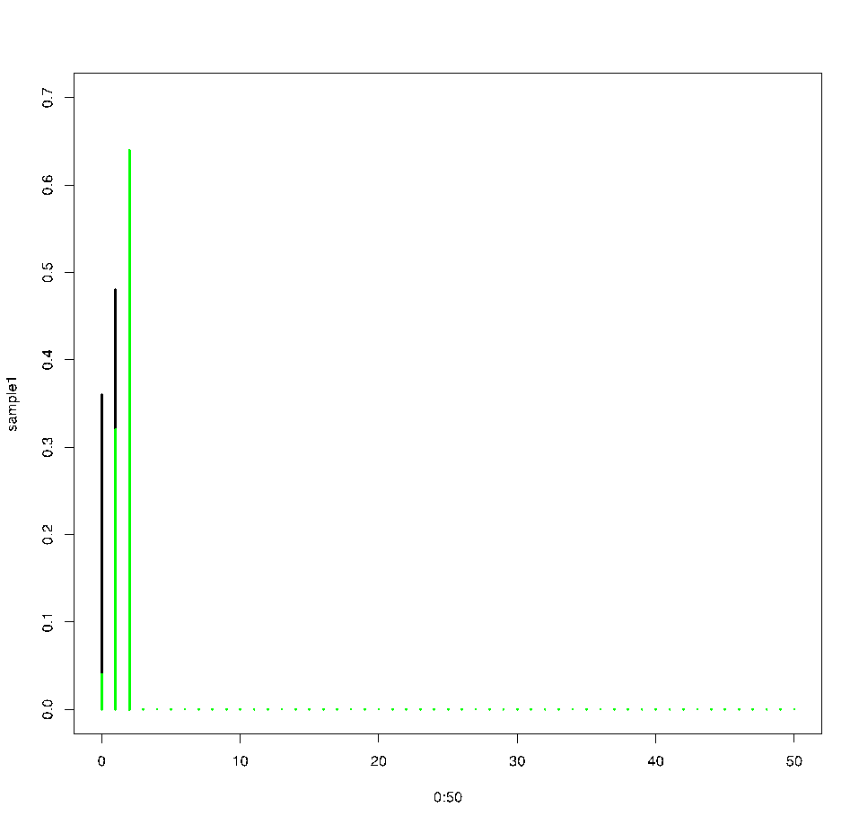
These two densities differ in their underlying probabilities of success (e.g. proportions of black balls in the set): the black one has success probability of 0.4, the green one 0.8. In this still plot we assumed that in both cases we have sampled only two balls. What would happen when we increase this number (the ‘size’ option in the ‘dbinom’ function)?
saveGIF({
for(i in 2:50){
## plot two binomial densities
sample1 <- dbinom(x = 0:50, size = 2, prob = 0.4)
plot(0:50, sample1, type=“h”, lwd=3, ylim=c(0,0.7))
sample2 <- dbinom(x = 0:50, size = i, prob = 0.8)
points(0:50, sample2, type=“h”, lwd=3, col=“green”)
## end of plot
}
}, interval = 0.1, ani.width = 550, ani.height = 550, movie.name=“binomial.gif”)
Here we again pasted the plotting block of code into the saveGIF loop. This time the ‘i' parameter changes from 2 to 50, i.e. within the range of possible sample sizes. In each step we assign this new ‘i' to the ‘size’ option. The outcome are two “sliding” binomial densities that move apart.
Identical principles can be used to visualize and animate data of any kind, including 3D plots produced through the ‘rgl’ or ‘scatterplot3D’ functions in R.
- Animations: not so difficult after all - October 12, 2016

